
Diversification lessons from the March quarter
The March 2020 quarter reminds us that the perception and the reality of portfolio diversification can turn out very different in adverse market environments. But that’s precisely when multi-asset investment portfolios need reliable diversification the most.
Many investments claim to offer diversification benefits only to end up highly correlated with equities on the downside and incurring outsized losses precisely when their advertised diversification benefits were most needed.
The lesson here is to look beyond asset class labels and focus instead on the underlying risk drivers that determine investment performance. To think about how those risk drivers will impact performance in different market environments and whether they are sufficiently different from the equity risk drivers that tend to dominate most multi-asset investment portfolios.
Viewing portfolio construction through the lens of underlying risk drivers leads to different conclusions, compared to focusing on asset class labels. The former leads to reliable diversification that delivers when most needed. The latter gives only the appearance of diversification.
Specifically in fixed income, watch out for investments that behave like defensive fixed income on the upside but more like equity investments on the downside. From a diversification perspective, that’s like an umbrella which only opens on sunny days. It fails to provide protection when most needed.
In this article we review the risk drivers of conventional fixed income investments – duration and credit – specifically from a multi-asset portfolio diversification perspective. We then evaluate how well they performed as diversifiers through the Q1 2020 turmoil.
The key takeaways from episodes like the March quarter?
- For reliably diversified portfolios, ignore asset class labels and focus instead on the underlying risk drivers of investments. Otherwise you end up just adding the same risks, only with different labels.
- Duration did OK as a diversifier for equity risk, but not nearly as well as it has in the past.
- Credit was a poor diversifier for equity risk, as it always has been.
- Despite labels, even ostensibly ‘safe’ investment grade credit has more in common with equities than defensive bonds, when viewed through the lens of underlying risk drivers.
To be clear, there is nothing inherently wrong with credit or duration based fixed income investments. Like any other investment, they come with certain risks in exchange for the returns they offer. Problems arise when they don’t behave as expected and fail to play the portfolio role they were supposed to.
Genuine and reliable risk diversification for multi-asset portfolios comes from adding investments whose underlying risk and return drivers are different to the conventional economic forces that dominate equity returns. Even better are investments that offer these attributes, while also maintaining a consistent volatility profile and reliable liquidity, irrespective of the market environment.
Best of all are investments that wrap all these attributes into a positively skewed return profile that offers additional performance upside when equities incur losses.
Multi-asset portfolio diversification concepts
The focus of this article is risk diversification in a multi-asset portfolio context, where the portfolio is invested across asset classes such as equities, fixed income, property, alternatives etc. This is intended to be a practical guide to key diversification concepts, rather than a rigorous academic analysis that delves into the nuances of optimal long-term strategic asset allocation.
In most cases, the objective of portfolio diversification is to reduce total portfolio volatility and mitigate the risk of extreme drawdowns. In most cases, equity risk tends to dominate multi-asset portfolio risk, therefore diversification is really about diversifying equity risk i.e. reducing total portfolio volatility and drawdown risk in scenarios where equities incur large losses.
As equities tend to have the highest expected returns over the long run, there is a trade-off here as portfolio diversification requires the inclusion of other types of investments into the portfolio, which may have lower expected returns (e.g. bonds).
Investors may therefore give up some expected return in exchange for reducing overall portfolio volatility. If done well, the reduction in expected return should be small relative to the reduction in portfolio volatility. If done really well, average portfolio volatility can be reduced while maintaining the same long run expected return. This is the holy grail. The so called ‘free lunch’ idea developed by Nobel prize winner Harry Markowitz.
Why should investors care about total portfolio volatility? Given the higher expected return of equities, why not just invest 100% in equities and ride the ups and downs? This comes down to things like individual risk appetite, the ‘volatility tax’ imposed by drawdowns on compounding returns and avoiding losses that can be terminal (i.e. a desire to ‘stay in the game’).
For example, think of two investment portfolios, each advertising an ‘average’ return of 10% per annum over the past two years. Portfolio A delivers +11% in year 1 and +9% in year 2. Portfolio B delivers -10% in year 1 and +30% in year 2. $100 invested in portfolio A would be worth $121 by the end of year 2. That same $100 invested in portfolio B would only be worth $117, even though portfolio B had the same ‘average’ return as portfolio A. That’s the volatility tax in action and it makes a big difference to long term compounded return outcomes.
Correlation
A key concept for portfolio diversification is correlation.
Rather than assessing investments on a purely standalone basis, the risk vs. return characteristics of each investment must be assessed in the context of how they interact with the other investments in the portfolio.
In an investing context, correlation is a commonly used measure of how returns from different investments move relative to one another. If the correlation is high, when one investment is incurring losses it’s likely the other will be too. If the correlation is low, you expect their returns to move independently of each other and if the correlation is negative, they generally move in opposite directions.
By combining uncorrelated or negatively correlated investments in a portfolio you can potentially diversify away some risk, without disproportionately reducing returns.
The classic example is the 60/40 balanced portfolio. It’s assumed that the 60% allocation to equities is uncorrelated (but ideally negatively correlated) to the 40% bond allocation, so when equities are down the bonds can generate gains to offset some of the equity losses and when equities are up, bonds are either stable or only incur small losses. This way your blended portfolio return is less volatile, and you end up with higher average returns per unit of volatility than if you held a 100% in equities.
In the same way this can be done with individual investments, it can also be done by combining uncorrelated funds.
This is a basic explanation of correlation that ignores important nuances and misconceptions that will surface later in this article. (further detail on correlation is available here and here)
The ideal diversifier
There are three main attributes via which an investment can reduce total portfolio volatility and mitigate the risk of extreme drawdowns, thereby helping to diversify equity risk in multi-asset portfolios:
Low volatility
Adding an explicitly low volatility investment will directly reduce average portfolio volatility, even if that investment is positively correlated with equities.
Low correlation
Adding a lowly correlated investment will reduce total portfolio volatility, even if that investment is still positively correlated with equities. The lower the correlation, the greater the potential for the investment to move independently of equities and therefore the stronger the volatility dampening effect at the total portfolio level. This effect is not dependent on the investment itself being low volatility in nature.
Negative correlation
The strongest portfolio volatility reduction benefit comes from adding a negatively correlated investment because it has the highest likelihood of moving in the opposite direction to equities and will therefore have the strongest volatility dampening effect. This effect is not dependent on the investment itself being low volatility in nature.
Consistency of behaviour is an important consideration. For example, an investment that exhibits low volatility and minimal correlation in benign market environments but then becomes highly volatile and positively correlated when equities fall is not an effective diversifier.
Ideal diversifiers combine all three of the above attributes and do so at the right time. For example, an investment that maintained consistently low volatility and minimal correlation to equities, irrespective of the market environment would be an effective diversifier. Even better would be one that maintained minimal correlation to equities in benign environments but actually becomes negatively correlated when equities fall (i.e. it has negative downside correlation / beta).
In addition to the above considerations, ideal risk diversifiers exhibit attractive standalone risk vs. return characteristics and do not cost a lot to hold. Cost could be explicit (e.g. paying for put options) or implicit (e.g. government bonds having lower expected returns than equities).
To summarise, an ideal diversifier would meet the following criteria:
- Reliably low volatility, irrespective of the market environment
- Reliably low correlation with equities, irrespective of the market environment.
- Evidence of negative downside correlation / beta, meaning it tends to generate positive returns when equities incur losses.
- Attractive standalone risk vs. return characteristics.
- Not costly to hold.
Given these multiple criteria for delivering reliable portfolio diversification benefits, it should be clear that conventional correlation alone is an insufficient metric. It’s important to consider other metrics like upside vs. downside volatility, downside capture, downside beta/correlation and how consistent they are through varying market environments.
Most importantly, one must understand the underlying risk drivers of different investments, consider how those risk drivers will impact performance in different market environments and decide whether they are sufficiently different from the equity risk drivers that tend to dominate most multi-asset investment portfolios.
The worst kinds of diversifiers are the ones that fail to deliver volatility dampening and/or correlation benefits when they are needed most (i.e. when equities fall a lot), and on top which they have poor risk vs return characteristics on a standalone basis.
These are pointless. Like an umbrella that only opens on sunny days.
Duration was an OK diversifier (but not like the good old days)
The interest rate duration exposure inherent in conventional government bond investments has long been the go-to diversifier of choice for multi-asset investment portfolios. (A refresher on duration is available here.)
The basic idea is that when equities fall, bond yields decline, resulting in capital gains on bond holdings, which help offset equity losses. In this way duration can help dampen overall portfolio performance volatility and reduce total portfolio level drawdown risk. The higher the starting point of bond yields (i.e. the yield cushion), the better this dynamic works.
Looking backward, we can point to historical episodes where duration has indeed worked very well as a defensive risk diversifier, with the best (relatively) recent example being the 2008 financial crisis (GFC). But since then, duration has been working less well.
As the table below shows, over subsequent equity drawdown periods following the GFC, the defensive protection provided by conventional government bond investments (i.e. duration) has progressively decreased as yield cushions shrunk. (These dynamics are explained in more detail here)
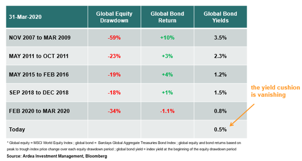
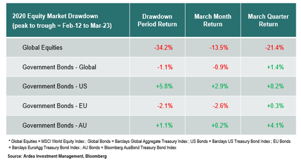
Q1 2020 saw the largest global equity market drawdown since the GFC and in some respects a more violent one. Against this backdrop, government bonds did not provide the same diversification benefits as they have in the past.
Evaluating duration over this period, against the desired attributes for an ideal diversifier, the results were OK, but not as great as they used to be.
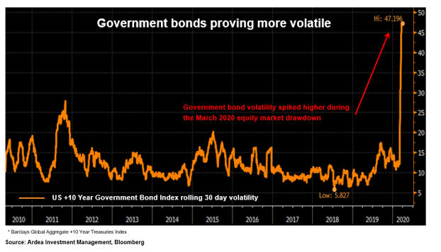
Low volatility criteria
Duration generally delivered on this criteria, but in many cases proved to be more volatile than they have been historically. This was particularly true for long dated government bonds, which carry the most duration risk. For example, the chart below shows the price volatility of a long-dated US government bond index.
Correlation criteria
On the correlation front, it depended on which particular government bonds you owned. As the table below shows, US and Australian government bonds exhibited decent negative downside correlation to equities, meaning they delivered profits as equities fell. However, global and European government bond indices were positively correlated with equities on the downside.
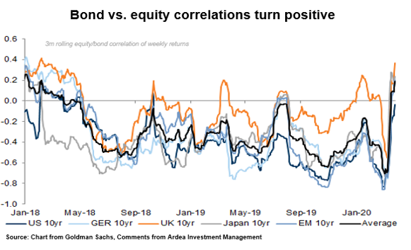
As the chart below shows, government bonds have generally been more positively correlated with equities than they have in the past, which is bad from a diversification perspective.
“For much of the past century, the building blocks of most investment portfolios have been a combination of riskier stocks and steadier, safer bonds. Like a see-saw, one typically rises if the other falls, smoothing returns and offering a hedge.
But over the past decade, this relationship has broken down. Bond yields have sagged as their prices have risen alongside equities, producing healthy gains but limiting how much protection bonds can offer in downturns. The recent market chaos unleashed by the coronavirus pandemic has underscored the problem, with bruising trading periods in which bonds and equities have dropped in unison.”
– Financial Times, ‘Market ructions test faith in classic portfolio mix’, April 2020
Why have government bonds and equities become more positively correlated? We can point to extreme central bank intervention across global financial markets as a recent cause (details here and here), while a longer history of bond vs. equity correlations shows substantial fluctuations across varying macroeconomic and policy regimes (details here).
Standalone risk vs. return and cost criteria
Duration scores poorly on this criteria. Ultra-low government bond yields have left duration exposure with very low expected returns (i.e. implicitly costly to hold) and an unfavourably asymmetric forward-looking risk vs return profile, while unprecedented fiscal stimulus creates the tail risk scenario of significant losses for duration exposure. (details here and here)
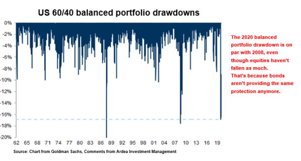
Even in the US, where duration performed best through the Q1 2020 turmoil, it was less effective as a portfolio diversifier than it has historically been.
“A [US] 60/40 portfolio had one of the largest drawdowns since the 1960s this month. This was due to the sharp equity drawdown but also as there was less of a buffer and diversification from bonds.
… In addition to the sharper-than-normal equity correction, diversification in 60/40 portfolios has been less good. First, with bond yields at all-time lows now and close to the effective lower bound, there is little space for most DM bonds to buffer equity drawdowns. In other words, the beta of bonds to equities has declined, especially in Europe and Japan. But also equity-bond correlations turned positive in most markets”
– Goldman Sachs, ‘The 60/40 Drawdown and Multi-Asset Portfolio Risk’, Mar 2020
The conclusions here are not binary. It’s not about which way bond yields will move from here or whether duration exposure should be excluded from portfolios entirely.
For multi-asset portfolios, it’s about a nuanced re-assessment of how government bonds are expected to behave, an objective scrutiny of how reliably duration exposure can continue to play its defensive role and balanced consideration of the tail-risk scenarios that might play out because of the unprecedented fiscal and monetary policy actions currently being implemented.
Credit was a poor diversifier (and always has been)
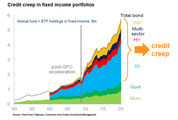
It’s only within the past decade that material credit risk has crept into defensive fixed income allocations. The traditional 60/40 balanced portfolio model specifically relied on high quality government bonds for their defensive attributes. Credit investments such as corporate bonds were not in the mix.
However, as collapsing interest rates intensified pressure on bond investors to boost returns, corporate bonds became the favourite sub-asset class within fixed income for yield hungry investors. As a result, there has been a pronounced ‘credit creep’ theme whereby even ‘defensive’ portfolios have persistently increased allocations to credit investments in pursuit of higher yields.
This credit creep theme can be seen in the chart below, which highlights the growing proportion of credit holdings in fixed income portfolios (labelled IG, HY, EM). The chart shows US specific data, but the same dynamics have played out globally.
In reference to credit creep, we previously noted:
“While these credit exposures have historically driven higher returns, they come at the cost of introducing equity beta into these portfolios, which compromises their diversification and downside protection benefits in adverse market environments.
This trade-off has become more important in the current environment because low yields make corporate bonds even more sensitive to equity market weakness.” (details here)
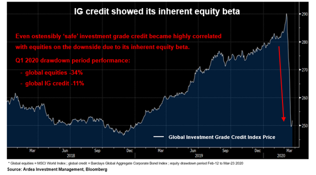
These dynamics played out in a big way during Q1 2020, when credit heavy fixed income portfolios suffered large losses as equities fell. To make matters worse, much of the credit investment universe also became highly illiquid, forcing many funds to impose large sell spreads. (details here)
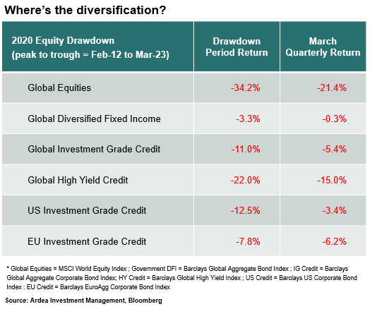
When assessing the above credit losses it’s important to do so in the context of the role those investments were supposed to play in a broader multi-asset portfolio.
It should be obvious that some segments of credit markets will get hit hard when equities fall (e.g. high yield, leveraged loans) and are therefore clearly not suitable for playing a defensive role. However, we find it’s underappreciated just how much ostensibly ‘safe’ investment grade / diversified fixed income investments can also fall and they often are used specifically to play a defensive role. It is in these cases where there was the greatest divergence between investors’ diversification expectations and the reality of what transpired.
“Many investors allocate to a bond fund with the broader portfolio in mind: that is not to make money in isolation but to protect capital and provide a counterweight to declines in holdings of stocks.
Government bonds do well in market panics for two reasons: one is that they are risk-free. Sovereigns are good for their money. The other is that in times of crisis central banks cut interest rates and buy bonds, pushing yields down and prices up.
But it seems too many bond funds had been chasing short term performance by loading up on corporate bonds that, like stocks, lose value in times of crisis. In effect, they traded away the insurance qualities of bonds in exchange for a modest increase in yield during the good times. When the crisis came these managers delivered lacklustre outcomes, particularly for investors that owned bonds for protection rather than profit.”
-AFR, “Bear with me: the cost of calling corrections”, April 30th
Evaluating credit over this period, against the desired attributes for an ideal diversifier, the results were poor.
Low volatility criteria
Credit failed on this criteria, becoming highly volatile on the downside. This is a consistent pattern of behaviour and is the worst kind of downside volatility trait because it surfaces when equities are also falling, which is precisely when it hurts a multi-asset portfolio most.
Correlation criteria
Credit failed on this criteria, becoming highly correlated with equities on the downside. We discuss this in more detail below.
Standalone risk vs. return and cost criteria
Prior to the Q1 2020 sell-off we noted that enormous yield chasing inflows to credit had pushed prices up to a point where the standalone risk vs. return trade-off in credit markets was generally very poor. (details here)
A consistent pattern of behaviour
Nothing that happened with credit in the March quarter is new, nor is it a temporary blip. This is a consistent pattern of behaviour that is entirely due to an undeniable structural feature of all credit investments – they have latent equity beta – and it becomes more pronounced when bond yields are low, as we previously noted:
“In the past, larger yield cushions gave corporate bonds a ‘get out of jail free’ card to help them ride through periods of equity market losses. Today, with yield cushions so small, the interest rate component is less able to provide that free pass when equities fall.
As a direct result of this, it’s prudent to expect the performance volatility and equity beta of corporate bonds to increase in adverse market environments going forward.
… Their equity sensitivity is latent in the sense that it’s hidden most of the time but can become very pronounced in adverse market environments, causing the largest losses for these portfolios when equities fall the most … precisely when the ‘defensiveness’ of fixed income is needed most.” (details here)
The events of Q1 2020 were driven by the same dynamics that play out every time equities experience a big drawdown. All credit investments become highly correlated with equities on the downside. It’s only the severity that varies across different segments of the credit universe, as Morningstar points out here with regard to the performance of credit during the GFC:
“Yields are so low, and credit-sensitive debt arguably so richly priced, that even if Treasury rates remain stable and low, economic trouble has plenty of potential to hurt riskier bonds.
Each of the following categories has an unusual factor or feature, but they all share the commonality of having some of the largest drawdowns during the financial crisis, taking a long time to recover, and having positive inflows thus far in 2019 and strong flows overall during the past five years.
U.S. Corporate Bond. More than 30 of the funds in today’s universe were around during the crisis as members of broader categories, and they didn’t fare well. On average they plunged more than 15% during the crisis from peak to trough.
… Multisector Bond. This category was among the worst hit during the crisis given the tendency of its funds to take more risk than core funds do in the pursuit of bigger yields and returns. So, when liquidity dried up, particularly among high-yield and emerging-markets sectors, this group took it on the chin. The category averaged a 19% drawdown, and even with the 2009 rally, it took nearly a year to recover.”
– Morningstar, ‘Handle these bond categories with care’, July 2019
Credit is where correlations can be most misleading
We noted earlier that conventional correlation calculations can be misleading when used in isolation and without a deeper analysis of the underlying risk drivers of an investment. The behaviour of credit investments provides a vivid illustration of this point, particularly investment grade (IG) credit.
IG credit returns can exhibit low (or even negative) correlation to equities in benign market environments but then become positively correlated when equities fall materially, as shown in the chart below.
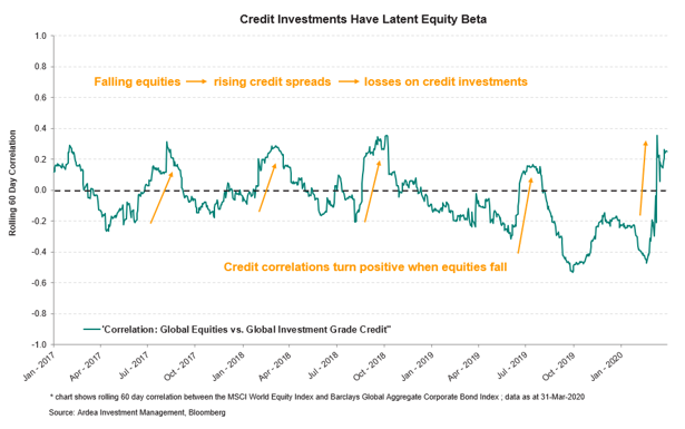
A basic correlation calculation can miss these nuances depending on the lookback window used for historical data and also because correlation assumes a linear relationship between the two variables. (details here)
More robust analysis spanning across economic cycles shows the positive correlation between corporate bond vs. equity prices is widely acknowledged across academic literature, as well as practitioner experience.
“The positive relationship between equity and corporate bond returns is also consistent with the Merton model and is by now a well-documented observation in the empirical literature (Cornell and Green, 1991; Shane, 1994; Reilly and Wright, 2001; Avramov, Jostova and Philipov, 2007).”
– Norges Bank: Corporate Bonds In A Multi-Asset Portfolio, Sep 2017
Why do IG credit correlations change in this way?
In benign environments IG credit tends to have low sensitivity to equity price movements. This is because the income component of credit returns dominates relative to corporate bond price fluctuations at these times, and the factors driving modest equity market fluctuations (e.g. corporate earnings, macroeconomic data) are not sufficient to materially change the perceived credit risk of high-quality IG companies. At these times the correlation of IG credit returns vs. equities will be low (or even negative).
However, in adverse market environments the same underlying risk drivers that cause equity losses become powerful enough to materially change the perceived credit risk of even the highest quality IG companies. At these times, the underlying fundamental links between equity and credit risk strengthen and the same risk drivers that hurt equity markets (e.g. weakening economic conditions, poor corporate earnings) also hurt bond markets’ perception of credit risk, leading to losses for credit investments as corporate bond prices drop. At these times the correlation of IG credit returns vs. equities increases materially, resulting in higher volatility and losses. (details here)
This changing nature of credit was clearly evident in the way credit behaved during the Q1 2020 global equity drawdown.
Through most of 2019, which was a positive equity market environment, credit behaved well, maintained low volatility and did not exhibit a strong positive correlation vs. equities. However, when the Q1 2020 sell-off hit, credit became highly volatile and correlated with equities on the downside, incurring substantial losses in the process. Mild-mannered Dr, Jekyll turned into the violent Mr. Hyde.
At these times, even IG credit portfolios that are highly diversified in the sense that they own a large number of corporate bonds issued by a diverse range of companies, still become highly correlated to the same few underlying risk drivers that are also hurting equity markets. A credit portfolio could contain a thousand different bonds but if all those bonds are impacted the same way by an economic downturn, there is little diversification of underlying risk drivers.
When viewed through the lens of underlying risk drivers, it becomes clear that credit heavy fixed income portfolios actually have more in common with equities than defensive bond investments. Therefore, from an asset allocation perspective, being long equities and being long credit represents very similar risk, just with different levels of volatility. So, whatever the label – investment grade, diversified fixed income, unconstrained, high yield, leveraged loans, private debt, ABS etc. – it’s all the same equity beta on the downside.
Focusing on asset class labels rather than underlying risk drivers results in weak and unreliable portfolio diversification. As such, for portfolios that already have material equity exposure, the diversification argument for adding credit is a weak one.
“… an allocation to corporate bonds has historically increased the overall volatility of multi-asset portfolios dominated by equity risk.”
– Norges Bank: Corporate Bonds In A Multi-Asset Portfolio, Sep 2017
In David Swensen’s influential book on portfolio management, the highly regarded head of Yale university’s endowment fund dismisses credit to an appendix titled ‘impure fixed income’. He argues that corporate bonds have little use from an asset allocation perspective because they don’t play a clear role. They don’t offer the genuine defensive protection of high-quality government bonds, nor do they offer the upside of equities.
He is being too harsh. While it should be clear that the diversification argument for adding credit to equity heavy multi-asset portfolios is weak. There may be other reasons for investing in credit. For example, as a tactical move to exploit particularly attractive standalone opportunities, as a lower beta equity replacement or as an income alternative to dividend paying stocks.
Whatever the use case, it’s important to be clear about what role credit investments are intended to play in a portfolio and whether their risk vs return and liquidity characteristics are optimal for reliably playing that role.
Implications for portfolio construction
The key lesson from the Q1 2020 turmoil is that traditional assumptions about multi-asset portfolio risk diversification are now proving less reliable.
Starting with duration
Ultra-low government bond yields mean vanishing yield cushions and inherently unfavourable asymmetry of duration risk. For these reasons duration can no longer be as effective a portfolio risk diversifier as it used to be.
We have now experienced two large equity drawdown episodes (Q4 2018 and Q1 2020) where conventional duration exposure failed to provide the kind of portfolio protection that it has in the past. These should be heeded as warning signs because they are not temporary blips. They represent a paradigm shift driven by vanishing yield cushions and the unfavourable asymmetry of duration risk.
While there is still a role for government bond beta exposure (i.e. duration) in multi-asset portfolios, particularly because it’s easy to understand and cheap to implement, it is a blunt instrument that works best when the starting point of bond yields is reasonably high. Access to a cheap beta exposure like duration can be attractive when that beta exposure offers an attractive risk vs. return proposition and can reliably play a portfolio role. Failing that it can be a false economy.
This is not to say that duration won’t work at all or that it should be abandoned entirely. Rather, the conclusion is that it is sub-optimal for multi-asset portfolios to be overly reliant on duration for risk diversification and downside protection vs. equity risk.
It’s time to look beyond the conventional duration lever to lesser known but increasingly compelling alternatives for defensive risk diversification. These can help fill the gap in scenarios where duration doesn’t work as well as hoped.
Turning to credit
We see a consistent pattern of behaviour whereby credit becomes volatile and positively correlated with equities on the downside every time equities experience a large drawdown. Combining these attributes with pronounced illiquidity risk makes credit investments poor risk diversifiers for multi-asset portfolios.
Even portfolios that hold ‘small’ allocations to credit can get hurt badly in severe equity market drawdowns because those small exposures exhibit high downside volatility in adverse environments, making them dominant drivers of portfolio returns and leading to outsized losses.
Looking beyond asset class labels and assessing credit through the lens of underlying risk drivers, it’s clear that credit has more in common with equities than reliably defensive bond investments and should therefore be considered that way from a portfolio construction perspective.
There’s a strong argument to be made that allocations to credit heavy investments should share the same risk budget as equities, rather than use up limited space in defensive allocations, given they were never suited to reliably play that defensive role in the first place.
The idea that defensive allocations ‘need’ to have credit because yields are so low is a red herring. For most multi-asset portfolios, the purpose of defensive allocations is to provide reliable diversification vs. equity risk, not to maximise yields (or income). If the aim is to maximise yield, that should be explicitly recognised and allocated to an appropriate part of the portfolio, rather than being slipped in under the cover of ‘diversification’.
And in conclusion
More generally, any investment that exhibits low volatility and low correlation vs. equities only in benign market environments, while becoming highly volatile and highly correlated with equities every time they fall, can hardly claim to be a good diversifier. It’s like an umbrella that only opens on sunny days.
To be clear, there is nothing inherently wrong with credit or duration based fixed income investments. Like any other investment, they come with certain risks in exchange for the returns they offer. Problems arise when they don’t behave as expected and fail to play the portfolio role they were supposed to.
What matters for achieving genuine and reliable risk diversification is considering how these exposures will behave in different scenarios, how those behaviours can change in varying market environments and how they will interact with other investments in the portfolio.
While the general concept of investment portfolio diversification is well known, the importance of focusing on underlying risk drivers rather than asset class labels is less well understood.
Genuine and reliable risk diversification for multi-asset portfolios comes from adding investments whose underlying risk and return drivers are different to the conventional economic forces that dominate equity returns. Even better are investments that offer these attributes, while also maintaining a consistent volatility profile and reliable liquidity, irrespective of the market environment.
Best of all are investments that wrap all these attributes into a positively skewed return profile that offers additional performance upside when equities incur losses.
This material has been prepared by Ardea Investment Management Pty Limited (Ardea IM) (ABN 50 132 902 722, AFSL 329 828). It is general information only and is not intended to provide you with financial advice or take into account your objectives, financial situation or needs. To the extent permitted by law, no liability is accepted for any loss or damage as a result of any reliance on this information. Any projections are based on assumptions which we believe are reasonable, but are subject to change and should not be relied upon. Past performance is not a reliable indicator of future performance. Neither any particular rate of return nor capital invested are guaranteed.